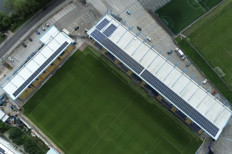
What set Alectrona apart was the documented design pack. We had quotes from three installers, but only Alectrona handed us a full set of drawings, a single-line diagram and a design referencing BS 7671 and the G99 connection process. The whole thing read like an engineering submission rather than a sales brochure. Our M&E consultant reviewed it and signed it off without a single query. That gave the board the confidence to release the capital.
Alectrona
Commercial guideWhy does commercial solar payback vary so much by sector?
Two identical arrays on identical roofs can pay back at very different rates, because payback tracks how much of the generation each building uses on site, and that self-consumption is set by how well a sector's demand lines up with the midday generation curve.
- Commercial scale, over 50 kWp
- On-site 3D drone survey + PV*SOL
- Engineer-led, outside MCS
The feedback we work to earn
These are representative example reviews, not yet-collected customer feedback. They are written to illustrate the kind of feedback Alectrona aims to earn and are shown as design placeholders while we gather and verify reviews from our first commercial clients. Alectrona is the commercial solar trading brand of RVTC LTD.
Other firms priced our roof off a satellite image and a desktop guess. Alectrona flew an in-house drone survey, fully insured and flown by a qualified commercial drone pilot, and built a 3D model of the actual roof. It picked up plant, vents and a parapet line that a flat aerial photo had completely missed, which changed the panel layout. I would rather find that out at design stage than on the day the scaffold goes up. The accuracy of that survey is the reason I trusted everything that followed.
As a finance director I was wary of being oversold a system bigger than we could use. Alectrona modelled the array against our actual half-hourly consumption data rather than an annual total, so it is sized to what we genuinely draw on site during the day. They were honest that exporting surplus is worth far less than self-consumption, and built the design around that. The capital case stacked up because the engineering was honest, not because the numbers were inflated.
We were undecided between buying outright, leasing and a PPA. Alectrona laid out all three side by side with the pros and cons of each against our balance sheet, instead of pushing the one that pays them best. They were clear about where a PPA makes sense and where capex wins, and pointed us at our own accountant for the tax treatment. The survey and design took a little longer than I expected, but the thoroughness was worth the wait. Genuinely consultative.
The install crew were tidy and well run, and worked to a clear CDM 2015 plan with a proper site induction and RAMS. What impressed me most was the handover. We received a full commissioning pack with the IEC 62446-1 test results, certification, O&M documentation and an as-built record for our maintenance team. As the people who have to live with this asset for the next twenty years, having that paperwork in order matters enormously. Nothing was left loose.
I expected the usual hard sell and got the opposite. After surveying our site Alectrona told us one roof section was not worth covering because of shading, and that a smaller, well-sited array was the better investment than filling every square metre. There was no commission-driven upselling and no pressure. For a six-figure capital project, that straight talk is exactly what you want from the people advising you. We will be using them again on our second site.
- Applies to Commercial systems over 50 kWp, outside MCS
- What drives it Self-consumption: how much generation the building uses on site
- Why sector matters It sets how well demand overlaps the midday generation curve
- Typical ranking Cold storage and manufacturing fast end; nine-to-five offices slower end
- The real figure Modelled per site from your half-hourly data, never a sector average
Payback by sector
People ask for a payback number by sector, and the honest answer is that the sector tells you the likely shape of the answer rather than the figure itself. For a system over 50 kWp, payback turns on one thing above roof size or panel count: how much of what the array generates the building uses on site, as it is produced, rather than exports. That share, self-consumption, is what the sector is really a proxy for, because each sector has a different demand profile relative to the solar generation curve.
This guide explains why payback varies by sector, how the common commercial sectors typically rank on profile match, and why the only honest figure for your site comes from modelling your real demand rather than a category average. It is a plain-English orientation for a finance or facilities director, not formal financial or tax advice; we confirm the specifics for your site from the survey and the PV*SOL model, and your accountant confirms the tax position.
Self-consumption against the generation curve
Solar output follows a daily bell curve that peaks around the middle of the day and falls to nothing overnight, and it is seasonal, strong from around April to September and weak from November to January in the UK. A unit generated is worth one of two very different things depending on what the building is doing at that moment. If the site is drawing power, the unit is self-consumed and offsets an expensive import unit, avoiding the energy cost plus the network and policy charges that ride on top of it. If the site is not drawing that power, the unit is exported and earns only the export rate, which is typically a fraction of the import rate.
So the single biggest lever on payback is how much of the generation curve overlaps your demand. A site with high, steady electrical load through daylight hours self-consumes most of what the array makes and pays back faster. A site whose demand sits outside those hours, or in one season, exports more of its generation and pays back slower unless storage or load-shifting is added. Sector is a proxy for that overlap, which is why the same kWp on two different buildings can return very differently. What decides it is the match between the demand profile and the generation profile, above the roof area or the panel count.
How the sectors typically rank on profile match
The sectors below are ordered by how well their demand usually lines up with daytime generation. This is the likely shape of the answer, not a guarantee, because every sub-sector and site differs.
- Cold storage and refrigerated logistics. The strongest match. Refrigeration compressors run around the clock with a large, near-constant baseload that fully overlaps the daylight generation curve, so a very high share is self-consumed with little export and little need for a battery. This sits at the fast end of the range.
- Manufacturing and process industry. A strong match where production runs through the day. Continuous or single-shift and double-shift loads from motors, compressed air, ovens and machinery create a high daytime baseload that overlaps generation well. Self-consumption is high for daytime-shift operations and falls for night-shift-heavy or intermittent batch processes.
- Retail and shops. Generally good daytime overlap, as trading-hours lighting, refrigeration, heating and cooling and tills coincide with daylight. Strongest for food retail, which carries a refrigeration baseload, and constrained mainly by available roof area on smaller units and by low overnight load.
- Warehousing and ambient logistics. Roof-rich but with a moderate match. Large roofs allow big arrays, but a non-refrigerated warehouse often has a modest baseload from lighting, materials-handling equipment charging and some heating and cooling, so a large array can outrun daytime demand and export the surplus. Electric vehicle or forklift charging and battery storage materially improve the match.
- Agriculture and horticulture. Highly seasonal and load-specific. Where daytime loads coincide with solar, such as summer irrigation and pumping, ventilation, grain drying, packhouse refrigeration or glasshouse loads, self-consumption is strong. Many farm loads are seasonal or off-peak, though, which depresses self-consumption unless paired with the right load or storage.
- Offices on a nine-to-five. The weakest match of these sectors. Demand concentrates in working hours but is comparatively low-intensity per square metre, drops at weekends and holidays, and has little overnight load, so a nine-to-five office self-consumes less of a given array and shows a longer payback than a high-baseload cold store when modelled on the same kWp.
Why the sector is a band, not a payback figure
The design implication is the honest takeaway: payback is modelled per site from that specific building's half-hourly consumption data against modelled generation for its roof. It is not a sector constant. The sector tells you the likely end of the range, the fast end for a cold store, the slower end for an office, but the actual figure depends on the individual load profile, the array sizing relative to that load, the import and export tariffs you actually pay, and whether a battery is added. No responsible payback figure can be quoted without the site's own consumption data, which is why we model your half-hourly demand against generation in PV*SOL before sizing anything rather than headline a number off a category average.
Self-consumption percentages quoted for sectors in solar marketing are directional at best, so we treat them as an ordering, cold storage ahead of manufacturing, manufacturing ahead of retail and warehousing, retail and warehousing ahead of offices, rather than as facts to print. Sub-sector matters too: food retail differs from non-food, arable from livestock from horticulture, daytime-shift manufacturing from night-shift. We read your actual profile rather than assume the band.
Where a battery shifts the answer
Storage changes the picture for sectors whose demand is misaligned with generation. A battery stores the midday surplus that would otherwise be exported cheaply and releases it into a later demand window, converting a low-value exported unit into a high-value avoided-import unit. That lifts self-consumption, and with it the return, for offices, ambient warehouses, evening-weighted retail and seasonal agriculture, the profiles that would otherwise spill the most generation to the grid.
Storage adds least where self-consumption is already high, such as a cold store or continuous manufacturing, because there is little surplus left to capture. So a battery is a lever we model on your real numbers and recommend only where it earns its place, rather than a default that overbuilds a system to export cheaply. The same half-hourly model that sets the array size tells us whether storage closes the gap on your profile or not, and we say so plainly either way.
How do your import and export tariffs change the sector ranking?
Self-consumption decides how much of the generation is valuable, but the import and export prices you actually pay decide how valuable each unit is, and that can reorder where a sector sits. A site on a high commercial import tariff captures a wider saving on every self-consumed unit than one on a cheaper contract, so two cold stores with identical profiles can show different paybacks purely on the tariff each negotiated. The spread between what you pay to import and what you earn to export is the real lever, and it is rarely the same for two businesses.
The structure of the tariff matters as much as the headline unit rate. Much of a large user's bill sits in the non-commodity charges layered on top of the wholesale price: the Distribution Use of System (DUoS) charges set by your network operator, which for Northern Powergrid in this region carry time-banded red, amber and green rates, plus transmission and policy costs. A unit of solar generated inside a weekday afternoon red band offsets the most expensive electricity of the day, so a sector whose load is heaviest then, such as a single-shift factory or a food retailer through trading hours, banks a larger saving per unit than the flat-rate comparison suggests. Ofgem sets the framework these charges run under, and the bands and rates are revised, so the live figures for your supply point come from your own bill and contract rather than a number printed here.
The same logic applies on the export side. Where you can secure a competitive Smart Export Guarantee or commercial power purchase agreement rate, the penalty for spilling surplus to the grid is smaller, which softens the disadvantage of a roof-rich, low-baseload profile like ambient warehousing. Where the export rate is poor, the case for sizing tightly to self-consumed load, or adding storage, sharpens. We model the design against the tariff you actually hold rather than a market average, and the wider economics, including how finance and tax sit on top, are set out under our commercial finance options and the ROI and payback guide.
What actually goes into the payback model behind a sector band?
A sector band is shorthand for the output of a model, and it helps to know what the model contains so the band is read for what it is. The generation side starts from how much a kilowatt of panels yields in a year on your roof, an annual kWh-per-kWp figure that depends on your latitude, orientation, pitch and shading, then discounts it by a performance ratio, typically modelled in the region of 0.80 to 0.85 to account for inverter, cable, temperature and soiling losses. These are PV*SOL starting points reconciled to your site, not promises, and we say which we used.
Against that generation curve the model overlays your half-hourly demand to find the self-consumed share, prices the self-consumed units at your import tariff and the surplus at your export rate, then projects both forward across the array's design life. A credible projection also carries an annual panel degradation allowance, so year-twenty output is lower than year-one, and it makes an assumption about how grid electricity prices move over time, which is itself uncertain. The payback period is where the cumulative saving overtakes the installed cost; the return can also be expressed as an internal rate of return or a net present value once a discount rate is applied. None of these are guarantees. They are modelled outcomes that move with tariff prices, generation in any given year and the assumptions fed in, which is why we present them as modelled and not promised, and why the tax treatment is confirmed by your accountant rather than asserted here.
The figure a sector band hides also has a boundary. A payback number reflects the array, its self-consumption and its tariffs; it does not by itself price in roof remediation, a constrained grid connection or storage, each of which can move the result. Those sit in their own analysis: the structural roof survey for roof condition, the connection assessment for any export cap, and the storage model where the profile spills surplus. Reading the band as a single clean number, rather than the output of these moving parts, is the mistake the band is meant to prevent.
Why can two sites in the same sector pay back differently?
The sector sets the likely shape, but the variation inside a single sector is wide enough that the label alone settles nothing. Shift pattern is the largest source of spread. A manufacturer running a single daytime shift sits high on profile match, because its machinery load lands squarely under the generation curve; the same factory on a night shift draws most of its power when the array makes nothing, so it self-consumes far less of an identical system and exports the daytime surplus. Weekend and holiday closures pull the same way: a five-day operation gives back roughly two days of weekly generation to low-value export, while a seven-day cold store or a continuous process does not.
Seasonality compounds it. UK generation is strong from around April to September and weak from November to January, so a load that is itself seasonal can align or clash with that curve. Summer-weighted demand, such as irrigation and ventilation in agriculture or cooling in a building that warms up in summer, overlaps peak generation and self-consumes well; a heating-led winter load misses it almost entirely. This is why a single sector spreads across a range rather than landing on a point, and why food retail with a refrigeration baseload separates cleanly from a non-food unit, or a daytime manufacturer from a night-shift one. The only way to place your building inside its sector's range is to read its own half-hourly profile, captured through your meter as the half-hourly metering guide describes, rather than assume the average. The sector is the band; your interval data is where on the band you actually sit.
Past the guide, this is how your figure actually gets set.
-
Survey On-site 3D drone survey
Our own insured pilot flies your roof and captures the real geometry and shading, so the design starts from your building instead of a satellite guess.
Booked to suit your operating hours
-
Model PV*SOL design and proposal
We model the array in bankable-grade software, size it around your daytime load, and set out generation, savings and payback across three funding routes.
Modelled, not promised
-
Install Engineered and installed
Designed and installed to BS 7671, commissioned to IEC 62446-1, connected under G99 and run under CDM 2015. Alectrona is typically the Principal Contractor.
Outside MCS, assured by the non-MCS stack
-
Aftercare Operations and maintenance
A 12-month defects period backed by an Insurance-Backed Guarantee, then ongoing operations and maintenance so the asset keeps earning for its full working life.
Kept performing, year on year
Indicative, not financial or tax advice. Confirm the position with a qualified accountant or tax adviser. Your figure comes from a survey-led PV*SOL model.
Last updated June 2026
Payback by sector: common questions
Because payback tracks self-consumption, and self-consumption depends on how well a sector's demand lines up with the solar generation curve. Solar peaks around midday and falls to nothing overnight, so a building with high, steady daytime load uses most of what the array makes and pays back faster, while one whose demand sits in the evening, the early morning or one season exports more and pays back slower. The same kWp returns differently on two buildings purely because of when their power is drawn.
The ones whose demand overlaps daytime generation most. Cold storage and refrigerated logistics sit at the fast end, because refrigeration runs around the clock with a large constant baseload that the array supplies directly. Daytime-shift manufacturing and food retail with a refrigeration baseload also match well. A nine-to-five office tends to sit at the slower end, because its load is lower-intensity and drops at weekends with little overnight demand. These are likely positions, not guarantees, and your figure comes from modelling your own load.
No, and it would be dishonest to try. Sector tells you the likely end of the range, but the actual figure depends on your individual load profile, the array sizing relative to that load, your import and export tariffs, and whether a battery is added. We model your half-hourly consumption against generation for your exact roof in PV*SOL before quoting anything. The sector is a band; your data is the answer. This is indicative orientation, not financial or tax advice; confirm the position with a qualified accountant or tax adviser.
The daytime case on its own is weaker, because generation peaks in the middle of the day, but it is not the end of the story. Where the load sits in the evening or overnight, a battery can store the midday surplus that would otherwise be exported cheaply and release it into that later window, lifting self-consumption and the return. We model that on your real numbers rather than overbuilding a roof that would export at a low rate, and where storage does not close the gap we say so honestly.
A self-consumed unit avoids the full import tariff you would otherwise pay, which is the energy cost plus the network and policy charges that ride on top of every imported unit. An exported unit earns only the export rate, typically a fraction of the import rate, set by the supplier or a commercial export agreement rather than the retail import price. Because the import-against-export spread is wide, every unit shifted from export to self-consumption is worth several times more, which is the economic engine behind the whole sector ranking.
We do not publish a price or a per-kWp figure, because a payback figure that is honest for your sector has to net a surveyed cost against your modelled, self-consumed saving rather than a headline number. Cost on a system over 50 kWp depends on roof type, mounting, inverter architecture, any grid-connection works and whether storage is added, so it is established from survey rather than quoted up front. Our commercial solar cost guide explains what drives the figure, and the finance options cover how the outlay is structured.
The honest answer needs at least twelve months of your half-hourly meter data, because the self-consumption that sets payback can only be read across a full year of both your demand and the seasonal generation curve. Once that data is to hand, modelling your profile against generation for your roof in PV*SOL and netting it against a surveyed cost is a matter of weeks. We confirm the timeline for your site at the start, and the modelled figure is presented as modelled rather than promised, with the tax position confirmed by your accountant.
Get the numbers for your roof.
A guide can only take you so far. The figure you get is modelled from your own half-hourly load and a system sized from the on-site drone survey. No obligation, and systems this size sit outside the domestic MCS scheme, so the assurance is the engineering stack.
- On-site 3D drone survey, fully insured in-house pilot
- Half-hourly load modelled in PV*SOL before anything is specified
- Engineer-led, assured to the non-MCS standard (CDM 2015)
- Capex, lease-purchase or PPA, whichever suits you